justify
key point
Law of Cosines
Law of Sines
left-multiply
line
| A | B | C | D | E | F | G | H | I | JKL | MN | O | P | Q | R | S | T | UV | WXYZ |
|---|---|---|---|---|---|---|---|---|---|---|---|---|---|---|---|---|---|---|
| Algebra 2 Connections Glossary | ||||||||||||||||||
justify |
|
|---|---|
| To give a logical reason supporting a statement or step in a proof. More generally to use facts, definitions, rules, and/or previously proven conjectures in an organized sequence to convincingly demonstrate that your claim is valid. (p. 109) | |
key point |
|
| An important point on a graph. Often an x- or y-intercept, a starting or ending point, a maximum or minimum point. Sometimes a point not on the graph that serves to locate an asymptote. (p. 9) | |
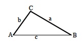
Law of Cosines |
|
| For any ∆ABC, a2 = b2 + c2 − 2bc cos A (pp. 28, 276)
|
|
Law of Sines |
|
| For any ∆ABC, |
|
left-multiply |
|
| Since multiplication of matrices is not commutative the product AB may not equal BA. If we start with matrix A and we want the product BA we must left‑multiply matrix A by matrix B. The order of the multiplication matters; therefore, we specify whether we are multiplying on the left side of the matrix or on the right, which would be right‑multiplying. (p. 366) | |
line |
|
| Graphed, a line is made up of an infinite number of points, is one-dimensional and extends without end in two directions. In two dimensions a line is the graph of an equation of the form ax + by = c . (pp. 11, 167, 190) | |
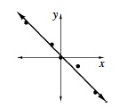
line of best fit |
|
| The line that best approximates several data points. For this course we place the line by visually approximating its position. An example is shown in the graph below.
|
|
line of symmetry |
|
A line that divides a figure into two congruent shapes which are reflections of each other across the line. (p. 167)
 |
|
linear equation |
|
| An equation with at least one variable of degree one and no variables of degree greater than one. The graph of a linear equation of two variables is a line in the plane. ax + by = c is the standard form of a linear equation. (p. 11) | |
linear function |
|
| A polynomial function of degree one or zero, with general equation f(x) = a(x − h) + k . The graph of a linear function is a line. (p. 38) | |
linear inequality |
|
| An inequality with a boundary line represented by a linear equation. (pp. 247, 326) | |
linear programming |
|
|---|---|
| A method for solving a problem with several conditions or constraints that can be represented as linear equations or inequalities. (pp. 241, 245) | |
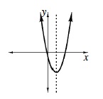
locator point |
|
| A locator point is a point which gives the position of a graph with respect to the axes. For a parabola, the vertex is a locator point. (p. 181) | |
locus |
|
| The location of a set of points that fit a given description. For example: A circle with center (5, –2) and radius 3 is described as the locus of points that are a distance of three units from the point (5, –2). (p. 566) | |
Log-Power Property |
|
| (p. 330) See “Power Property of Logs.” | |
Log-Product Property |
|
| (pp. 334, 335) See “Product Property of Logs.” | |
Log-Quotient Property |
|
| (pp. 334, 335) See “Quotient Property of Logs.” | |
logarithm |
|
| An exponent. In the equation y = 2x, x is the logarithm, base 2, of y, or log2y = x. (pp. 282, 283) | |
logarithmic and exponential notation |
|
| m = logb(n) is the logarithmic form of the exponential equation bm = n(b > 0) (). (p. 283) | |
logarithmic functions |
|
| Inverse exponential functions. The base of the logarithm is the same base as that of the exponential function. For instance y = log2x can be read as “y is the exponent needed for base 2 to get x,” and is equivalent to x = 2y. The short version is stated “log, base 2, of x,” and written log2x. (pp. 281, 285, 286) | |